Activity 16: Image Segmentation

September 2, 2008 at 11:12 am (Uncategorized)

Segmentation (choosing of objects in colored images) is useful in many aspects of digital image processing like face detection. More often than not, an object would have one color, for example, a mug or a ball, or hand. However, lighting variations may affect the luminosity of our images and as such, we must remove these luminosity attributes in processing our images. To remove luminosity effects we normalized each channel to

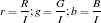
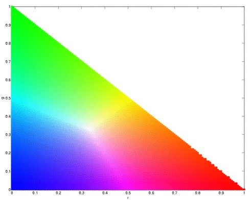
where . We then crop a portion of the object (regions of interest, ROI) that we will segment and use this as a “model” from which certain parameters will be obtained. If our object is more or less monochromatic, it will more or less cover a small blob in our chromaticity diagram (figure above). We then. Here, we have a picture of Catherin Zeta-Jones taken from: http://www.latest-hairstyles.com/

Our “model” is a patch form here neck down to her bust to gather as much colors as possible.

Parametric Probability Distribution

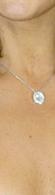
We assume that the distribution of colors in our ROI are normally distributed where the mean and the variance we obtain from our “model” cropped images. The probability that the red channel of a pixel is belonging to the red component of the “model” is given by

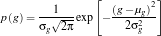
where and are the mean and standard deviation respectively. The probability that a pixel belongs to the “model” is a joint probability given by

We perform this over all pixels and plot the probability that a pixel belongs to our ROI.

Here is our distrution but is not yet normalized.

We obtained the joint probability distribution and used “imshow” to plot the probability that a pixel belongs to our ROI. As we can see, most of her torso, face and neck is colored almost white, which means there is high probability that hey belong to our ROI. And advantage of this method is it is more robust when it comes to color of the ROI not belonging to the “model”.

Non-parametric Probability Distribution (Histogram Backprojection)

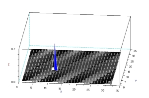
The next method is through histogram backprojection. In this method, we used a normalized chromaticity distribution histogram (obtained from the “model”) with 32 bins along the red and green. The histogram of the model is shown below.

This method works by getting the r and g values of a pixel and locates the probabilty that it belongs to the “model”. It replaces the pixel value with the probility of the pixel r-g values. The reconstruction is shown below.

As can be seen, this has better segmentation of the face, torso and arms. Another advantage of this method is it doesn’t assume normality of distribution unlike parametric one.

<!–

Extra Extra!

Furthermore, I applied what we have learned in Activity 3 and Activity 9 in this activity. I threshold the image to get a black and white image, resulting to this:

Looking closely, there are speckles in the hair, so i improved it by opening transformation and obtained this image

–>

-oOo-

clear all;
stclear all;
stacksize(4e7);
chdir(‘/home/jeric/Documents/Acads/ap186/a16’);
ROI=imread(‘face.jpg’);
I=ROI(:,:,1)+ROI(:,:,2)+ROI(:,:,3);
I(find(I==0))=100;
ROI(:,:,1)=ROI(:,:,1)./I;
ROI(:,:,2)=ROI(:,:,2)./I;
ROI(:,:,3)=ROI(:,:,3)./I;

ROI_sub=imread(‘face_cropped.jpg’);
I=ROI_sub(:,:,1)+ROI_sub(:,:,2)+ROI_sub(:,:,3);
ROI_sub(:,:,1)=ROI_sub(:,:,1)./I;
ROI_sub(:,:,2)=ROI_sub(:,:,2)./I;
ROI_sub(:,:,3)=ROI_sub(:,:,3)./I;

//probability estimatation
mu_r=mean(ROI_sub(:,:,1)); st_r=stdev(ROI_sub(:,:,1));
mu_g=mean(ROI_sub(:,:,2)); st_g=stdev(ROI_sub(:,:,2));

Pr=1.0*exp(-((ROI(:,:,1)-mu_r).^2)/(2*st_r^2))/(st_r*sqrt(2*%pi));
Pg=1.0*exp(-((ROI(:,:,2)-mu_g).^2)/(2*st_g^2))/(st_r*sqrt(2*%pi));
P=Pr.*Pg;
P=P/max(P);
scf(1);
x=[-1:0.01:1];
Pr=1.0*exp(-((x-mu_r).^2)/(2*st_r))/(st_r*sqrt(2*%pi));
Pg=1.0*exp(-((x-mu_g).^2)/(2*st_g))/(st_g*sqrt(2*%pi));
plot(x,Pr, ‘r-‘, x, Pg, ‘g-‘);

scf(2);
imshow(P,[]);
//roi=im2gray(ROI);
//subplot(211);
//imshow(roi, []);
//subplot(212);

//<————-histogram backprohection————————————>
//histogram
r=linspace(0,1, 32);
g=linspace(0,1, 32);
prob=zeros(32, 32);
[x,y]=size(ROI_sub);
for i=1: x
for j=1:y
xr=find(r<=ROI_sub(i,j,1));
xg=find(g<=ROI_sub(i,j,2));
prob(xr(length(xr)), xg(length(xg)))=prob(xr(length(xr)), xg(length(xg)))+1;
end
end
prob=prob/sum(prob);
//show(prob,[]); xset(“colormap”, hotcolormap(256));
scf(3)
surf(prob);

//backprojection
[x,y]=size(ROI);
rec=zeros(x,y);
for i=1: x
for j=1:y
xr=find(r<=ROI(i,j,1));
xg=find(g<=ROI(i,j,2));
rec(i,j)=prob(xr(length(xr)), xg(length(xg)));
end
end
scf(4);
imshow(rec, []);
rec=round(rec*255.0);
getf(‘imhist.sce’);
[val, num]=imhist(rec);
scf(5);
plot(val, num);
scf(6);
rec=im2bw(rec, 70/255);
imshow(rec, []);

//opening
se=ones(3,3);
im=rec;
im=erode(im, se);
im=dilate(im, se);
scf(7);
imshow(im, []);

-oOo-

I give myself a 10 here because I did well in segmenting the images. 🙂