Activity 18: Minimum Distance Classification
Pattern recognition techniques has long been studied by scientists for their potential applications. Human face recognition, coral reef analysis and gait analysis have been successful implentations of pattern recognition techniques.
One of the most basic forms of pattern recognition techniques is through attibutes of a given sample and compare it with the attributes of a training set. In this activity, we use different samples of chips, namely Chippy, Nova and Piatos and attempted to distinguish chips from each other through the attributes obtained form the training set.

Ten samples of each kind of chip was photographed with a camera. After which, cut each images to ascertain that a single image contains a single chip. Image processing techniques such segmentation was performed to remove the chip from the background. Afterwich the average value of the R, G and B of each chip was obtained as well as the area. The chip is then represented by the vector x containing the features of the chip. We do this for all chips in our training set. If we have W types of chips (chippy, nova, and piatos), we obtain the average feature vector of each class given by

for all j=1,2,..W.
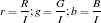
The features of each test chip are obtained and the distance from each class is computed using

where

The test chip is classified based on the class with the minimum distance. Take note also that I normalized each vector to eliminate bias towards features whose values are extremely large (area for example) and eliminate bias against small numbers (R value for example).
Here is the confusion matrix of the test set of my 3-class classification. This is good enough with accuracy of 87%.

Activity 17: Basic Video Processing
Videos are becoming common with the advent of the digital era. Almost anyone can create their own videos. We can take advantage of this technology in exploring physics by performing experiments and monitor certain variables as a function of time.
A video is simply a string of still images flashed one after the other. The rate at which the video is captured is called the frame rate (measured in frames per second, fps). The higher the frame rate, the higher quality of the image in terms of smoothness of motion and time resolution. In our case, we used Cole’s web camera that can capture videos to see the dynamics of a physical pendulum (as opposed to a simple pendulem). His camera has frame rate of 15fps and, by Nyquist criterion, we can only resolve harmonic motion with frequency of less than 8Hz.
In this activity our group (me, cole and mark) decided that we want to invsitigate the period of a physical pendulum and compare it with theoretical predictions. For the first part, we captured video from the web cam and converted the frames to image files in *.jpg format (using avidemux) with the same fps but with reduced images size to 120 by 180 (from the original 480 by 720). The images were then subject to white balancing, chromaticity normalization, image segmentation (using color), binarization (using grayscale histogram), and opening and closing transformation. Basically we applied here everything we did for the entire sem. :). Assumptions regarding the ruler include homogeneity in the density of the ruler, the pivot is at excatly at the edge, and that the center of mass located exactly in the middle of the ruler.

Here is the gif animation i made (i converted the images to gif animation to avoid problems with the UP blocking access to video sharing sites such as youtube). The left is the orginal set of images, the middle are the normalized ones and the last are the binarized images. The gif is quite large (1.6mb) but once it gets loaded, it keeps on rolling. 🙂 I also ensured the the speed of the gif is similar to the fps of the camera used.
A physical pendulum is a more generalized pendulum with no ideal strings. The period of oscillation of this pendulum is given by

where I is the moment of inertia about the pivot and L is the distance of the center of mass from the pivot. 
For our ruler with length h and width w with pivot around the end the moment of inertia is given by

The period of oscillation can be obtained from the graph by plotting the location of the center of mass as a function of time and getting the distance between two peaks.If this is what we use, we get a period of 1.2 sec

I also used fft to get the dominating frequency of our signal above, and found it to 0.769 Hz or a period of around 1.3 sec which is not far from the above. I also believe that the frequency obtained by fft is more accurate than just picking peaks. 🙂

Theoretically, this ruler with mass 174.8g, length of 63.5cm and width of 3cm would have a period of oscillation of 1.31s (the moment of inertia being 0.0235). This means we have error of only 0.76%. This is very near the expected value , considering that the we had a few assumptions regarding this ruler.
-oOo-


-oOo-
Here are the functions i made that were invoked above.
closing.sce

open.sce

imhist.sce

segment.sce

white_balance.sce

-oOo-
Collaborators: Mark, Cole
I want to give myself a 10 here because i believe I was able to complete what has to be done by applying almost everything we had learned.:)
Activity 16: Image Segmentation
Segmentation (choosing of objects in colored images) is useful in many aspects of digital image processing like face detection. More often than not, an object would have one color, for example, a mug or a ball, or hand. However, lighting variations may affect the luminosity of our images and as such, we must remove these luminosity attributes in processing our images. To remove luminosity effects we normalized each channel to
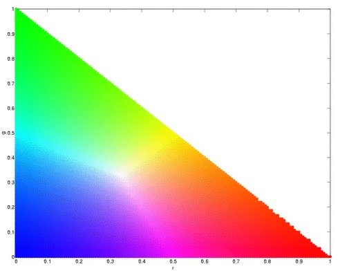
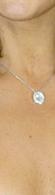
where  . We then crop a portion of the object (regions of interest, ROI) that we will segment and use this as a “model” from which certain parameters will be obtained. If our object is more or less monochromatic, it will more or less cover a small blob in our chromaticity diagram (figure above). We then. Here, we have a picture of Catherin Zeta-Jones taken from: http://www.latest-hairstyles.com/

Our “model” is a patch form here neck down to her bust to gather as much colors as possible.
Parametric Probability Distribution
We assume that the distribution of colors in our ROI are normally distributed where the mean and the variance we obtain from our “model” cropped images. The probability that the red channel of a pixel is belonging to the red component of the “model” is given by
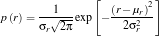
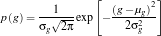
where  and
and  are the mean and standard deviation respectively. The probability that a pixel belongs to the “model” is a joint probability given by

We perform this over all pixels and plot the probability that a pixel belongs to our ROI.
Here is our distrution but is not yet normalized.
We obtained the joint probability distribution and used “imshow” to plot the probability that a pixel belongs to our ROI. As we can see, most of her torso, face and neck is colored almost white, which means there is high probability that hey belong to our ROI. And advantage of this method is it is more robust when it comes to color of the ROI not belonging to the “model”.
Non-parametric Probability Distribution (Histogram Backprojection)
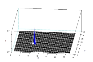
The next method is through histogram backprojection. In this method, we used a normalized chromaticity distribution histogram (obtained from the “model”) with 32 bins along the red and green. The histogram of the model is shown below.
This method works by getting the r and g values of a pixel and locates the probabilty that it belongs to the “model”. It replaces the pixel value with the probility of the pixel r-g values. The reconstruction is shown below.
As can be seen, this has better segmentation of the face, torso and arms. Another advantage of this method is it doesn’t assume normality of distribution unlike parametric one.
<!–
Extra Extra!
Furthermore, I applied what we have learned in Activity 3 and Activity 9 in this activity. I threshold the image to get a black and white image, resulting to this:
Looking closely, there are speckles in the hair, so i improved it by opening transformation and obtained this image
–>
-oOo-
clear all;
stclear all;
stacksize(4e7);
chdir(‘/home/jeric/Documents/Acads/ap186/a16’);
ROI=imread(‘face.jpg’);
I=ROI(:,:,1)+ROI(:,:,2)+ROI(:,:,3);
I(find(I==0))=100;
ROI(:,:,1)=ROI(:,:,1)./I;
ROI(:,:,2)=ROI(:,:,2)./I;
ROI(:,:,3)=ROI(:,:,3)./I;
ROI_sub=imread(‘face_cropped.jpg’);
I=ROI_sub(:,:,1)+ROI_sub(:,:,2)+ROI_sub(:,:,3);
ROI_sub(:,:,1)=ROI_sub(:,:,1)./I;
ROI_sub(:,:,2)=ROI_sub(:,:,2)./I;
ROI_sub(:,:,3)=ROI_sub(:,:,3)./I;
//probability estimatation
mu_r=mean(ROI_sub(:,:,1)); st_r=stdev(ROI_sub(:,:,1));
mu_g=mean(ROI_sub(:,:,2)); st_g=stdev(ROI_sub(:,:,2));
Pr=1.0*exp(-((ROI(:,:,1)-mu_r).^2)/(2*st_r^2))/(st_r*sqrt(2*%pi));
Pg=1.0*exp(-((ROI(:,:,2)-mu_g).^2)/(2*st_g^2))/(st_r*sqrt(2*%pi));
P=Pr.*Pg;
P=P/max(P);
scf(1);
x=[-1:0.01:1];
Pr=1.0*exp(-((x-mu_r).^2)/(2*st_r))/(st_r*sqrt(2*%pi));
Pg=1.0*exp(-((x-mu_g).^2)/(2*st_g))/(st_g*sqrt(2*%pi));
plot(x,Pr, ‘r-‘, x, Pg, ‘g-‘);
scf(2);
imshow(P,[]);
//roi=im2gray(ROI);
//subplot(211);
//imshow(roi, []);
//subplot(212);
//<————-histogram backprohection————————————>
//histogram
r=linspace(0,1, 32);
g=linspace(0,1, 32);
prob=zeros(32, 32);
[x,y]=size(ROI_sub);
for i=1: x
for j=1:y
xr=find(r<=ROI_sub(i,j,1));
xg=find(g<=ROI_sub(i,j,2));
prob(xr(length(xr)), xg(length(xg)))=prob(xr(length(xr)), xg(length(xg)))+1;
end
end
prob=prob/sum(prob);
//show(prob,[]); xset(“colormap”, hotcolormap(256));
scf(3)
surf(prob);
//backprojection
[x,y]=size(ROI);
rec=zeros(x,y);
for i=1: x
for j=1:y
xr=find(r<=ROI(i,j,1));
xg=find(g<=ROI(i,j,2));
rec(i,j)=prob(xr(length(xr)), xg(length(xg)));
end
end
scf(4);
imshow(rec, []);
rec=round(rec*255.0);
getf(‘imhist.sce’);
[val, num]=imhist(rec);
scf(5);
plot(val, num);
scf(6);
rec=im2bw(rec, 70/255);
imshow(rec, []);
//opening
se=ones(3,3);
im=rec;
im=erode(im, se);
im=dilate(im, se);
scf(7);
imshow(im, []);
-oOo-
I give myself a 10 here because I did well in segmenting the images. 🙂
