Activity 15: White Balancing

August 28, 2008 at 11:07 am (Uncategorized)

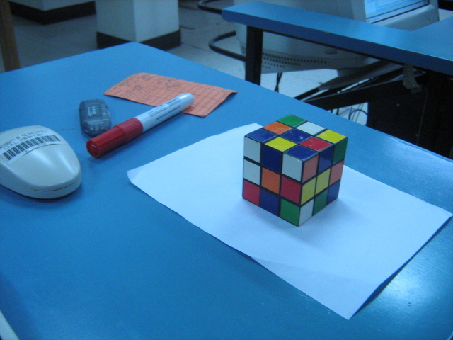
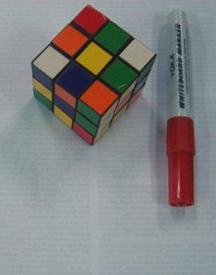
White balancing is a technique wherein in images captured under lighting conditions are corrected such that white appears white. It may not really be obvious (since the eyes have white balancing capabilities) unless we compare the object with the image itself. Here is an image of a rubix cube take under different white-balancing conditions in a room with fluorescent light.

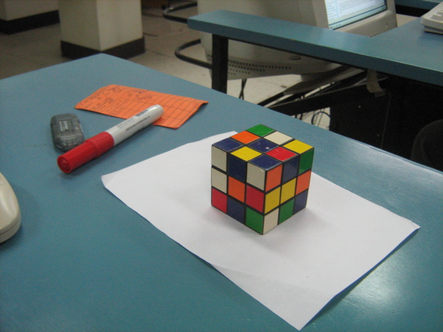
Automatic white balancing.

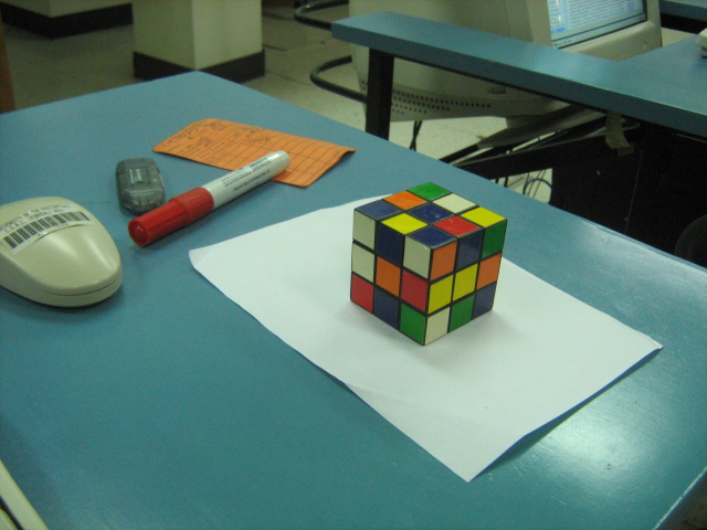
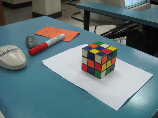
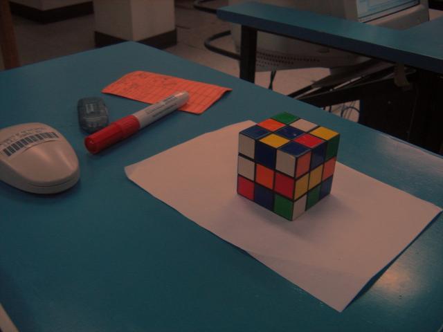
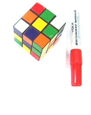
cloudy, daylight and fluorescent white balancing

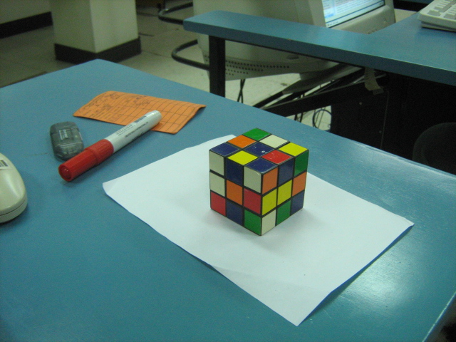
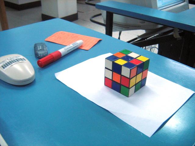
tungsten white balancing

From the images above, we can see that if you just used any white balance, we may not get the desired image. And can be seen in the case of tungsten, white doesn’t appear white.This can be corrected via white balancing methods. There are two methods that can be used in performing white balancing, namely, the Reference White and the Gray World algorithm.

Let’s start with the basic. A digital image is composed of an MxNx3 matrix where MxN is the dimension of the image and there are 3 channels for that image. Each channel corresponds to one of the three primary colors namely red, green and blue. A pixel then is contains the information about the amount of red, green and blue in that channel. The reference white algorithm works by choosing a white object in the image and getting it’s RGB values. This is used as reference for determining which is “white” in the image. The red channels of each pixel is divided by the red value of the reference white object. The same is done for all other channels. The gray world algorithm on the other hand works by assuming the image is gray (ie, each pixel has equal R-G-B values).The gray world algorithim is implemented by averaging the R-G-B of each channel in the unbalanced image. The red channel of the unbalanced image is then divided by the R above. The same is done for the blue and green channels. If a channel exceeds 1.0 on any pixel, it is cut-off to 1.0 to avoid saturation.

Here is the result of white balancing using the gray world algo (left) and the reference white (right). As can be seen here, can see that reference white is superior in terms of image quality. The problem with GWA is that averaging channels puts bias to colors that are not abundant. In our case, there is bias against the green.

Here we tried to implement GWA and RW by making the background white to ensure more or less the same amount of colors present.

Here is the results for GWA (left) and RF (right). The rendering of white of GWA is OK, and is close to the actual image. On the other hand, the RF method produced a very brightly colored image. Now, we can see that a disadvantage of RF is that it relies on what should be white and is highly subjective then. A problem would exist in RF if there are no white objects in the image (or if a reference white is not exactly white).

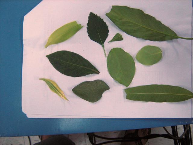
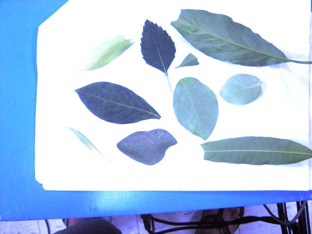
Here we used many shades of green in performing white balancing.

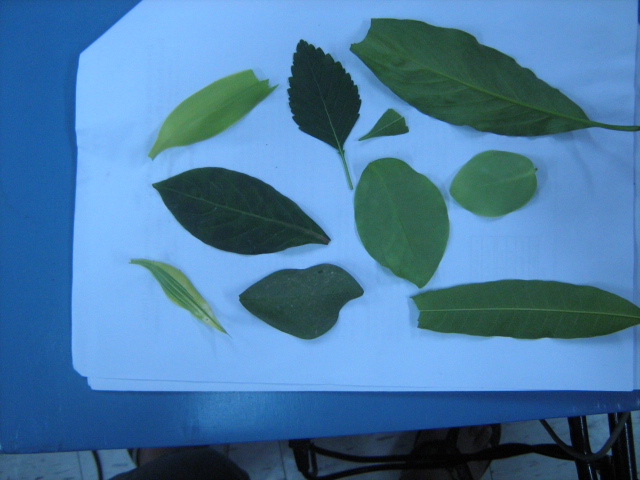
We can see that the GWA produced better results than RF. Again, RF saturated with the white.

I give myself a 10 for this activity.

-oOo-

clear all;
stacksize(4e7);
name=’leaf_and_all 001‘
im=imread(strcat(name + ‘.jpg’));
//imshow(im);
//[b,xc,yc]=xclick()
//reference white
x=124;
y=184;
r=im(x,y,1);
g=im(x,y,2);
b=im(x,y,3);
im1=[];
im1(:,:,1)=im(:,:,1)/r;
im1(:,:,2)=im(:,:,2)/g;
im1(:,:,3)=im(:,:,3)/b;
g=find(im1>1.0);
im1(g)=1.0;
imwrite(im1, strcat(name + ‘rw.jpg’));
//imshow(im,[]);

//grayworld
r=mean(im(:,:,1));
g=mean(im(:,:,2));
b=mean(im(:,:,3));
im2=[]
im2(:,:,1)=im(:,:,1)/r;
im2(:,:,2)=im(:,:,2)/g;
im2(:,:,3)=im(:,:,3)/b;
im2=im2/max(im2);
g=find(im2>1.0);
im2(g)=1.0;
imwrite(im2, strcat(name + ‘gw.jpg’));
//imshow(im,[]);