Activity 15: White Balancing
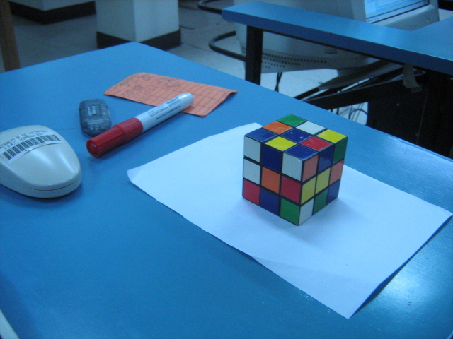
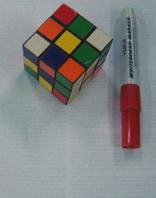
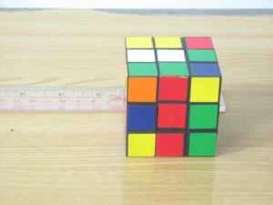
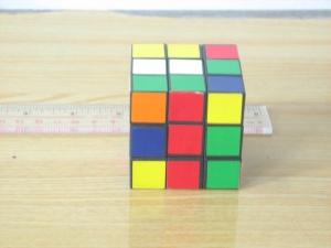
White balancing is a technique wherein in images captured under lighting conditions are corrected such that white appears white. It may not really be obvious (since the eyes have white balancing capabilities) unless we compare the object with the image itself. Here is an image of a rubix cube take under different white-balancing conditions in a room with fluorescent light.
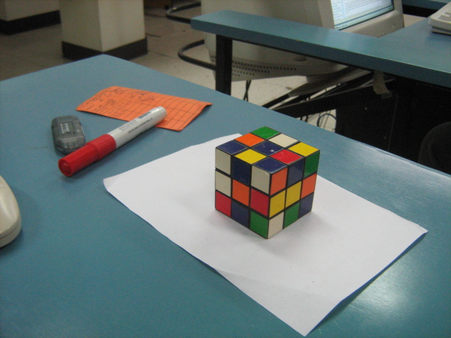
Automatic white balancing.
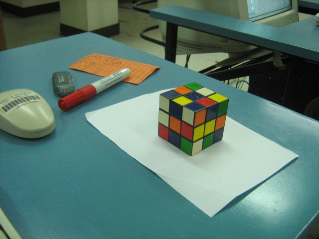
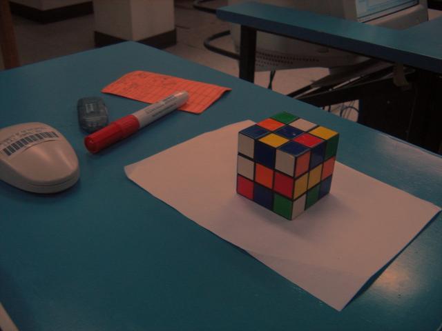
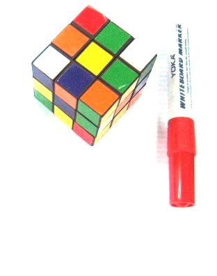
cloudy, daylight and fluorescent white balancing
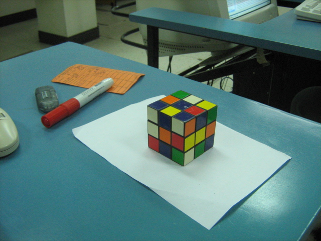
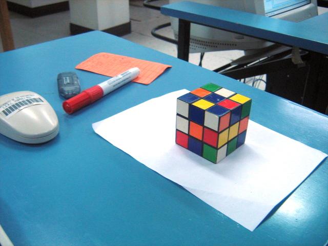
tungsten white balancing
From the images above, we can see that if you just used any white balance, we may not get the desired image. And can be seen in the case of tungsten, white doesn’t appear white.This can be corrected via white balancing methods. There are two methods that can be used in performing white balancing, namely, the Reference White and the Gray World algorithm.
Let’s start with the basic. A digital image is composed of an MxNx3 matrix where MxN is the dimension of the image and there are 3 channels for that image. Each channel corresponds to one of the three primary colors namely red, green and blue. A pixel then is contains the information about the amount of red, green and blue in that channel. The reference white algorithm works by choosing a white object in the image and getting it’s RGB values. This is used as reference for determining which is “white” in the image. The red channels of each pixel is divided by the red value of the reference white object. The same is done for all other channels. The gray world algorithm on the other hand works by assuming the image is gray (ie, each pixel has equal R-G-B values).The gray world algorithim is implemented by averaging the R-G-B of each channel in the unbalanced image. The red channel of the unbalanced image is then divided by the R above. The same is done for the blue and green channels. If a channel exceeds 1.0 on any pixel, it is cut-off to 1.0 to avoid saturation.
Here is the result of white balancing using the gray world algo (left) and the reference white (right). As can be seen here, can see that reference white is superior in terms of image quality. The problem with GWA is that averaging channels puts bias to colors that are not abundant. In our case, there is bias against the green.
Here we tried to implement GWA and RW by making the background white to ensure more or less the same amount of colors present.
Here is the results for GWA (left) and RF (right). The rendering of white of GWA is OK, and is close to the actual image. On the other hand, the RF method produced a very brightly colored image. Now, we can see that a disadvantage of RF is that it relies on what should be white and is highly subjective then. A problem would exist in RF if there are no white objects in the image (or if a reference white is not exactly white).
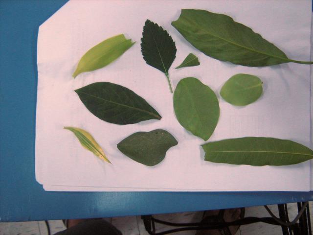
Here we used many shades of green in performing white balancing.
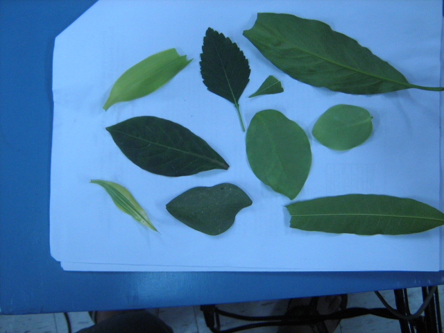
We can see that the GWA produced better results than RF. Again, RF saturated with the white.
I give myself a 10 for this activity.
-oOo-
clear all;
stacksize(4e7);
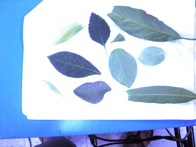
name=’leaf_and_all 001‘
im=imread(strcat(name + ‘.jpg’));
//imshow(im);
//[b,xc,yc]=xclick()
//reference white
x=124;
y=184;
r=im(x,y,1);
g=im(x,y,2);
b=im(x,y,3);
im1=[];
im1(:,:,1)=im(:,:,1)/r;
im1(:,:,2)=im(:,:,2)/g;
im1(:,:,3)=im(:,:,3)/b;
g=find(im1>1.0);
im1(g)=1.0;
imwrite(im1, strcat(name + ‘rw.jpg’));
//imshow(im,[]);
//grayworld
r=mean(im(:,:,1));
g=mean(im(:,:,2));
b=mean(im(:,:,3));
im2=[]
im2(:,:,1)=im(:,:,1)/r;
im2(:,:,2)=im(:,:,2)/g;
im2(:,:,3)=im(:,:,3)/b;
im2=im2/max(im2);
g=find(im2>1.0);
im2(g)=1.0;
imwrite(im2, strcat(name + ‘gw.jpg’));
//imshow(im,[]);
Activity 14: Stereometry
here is the RQ factorization code from: http://www.cs.nyu.edu/faculty/overton/software/uncontrol/rq.m written by Michael Overton and modified by yours truly for scilab.
-oOo-
function [R,Q]= rq(A)
//% full RQ factorization
//% returns [R 0] and Q such that [R 0] Q = A
//% where R is upper triangular and Q is unitary (square)
//% and A is m by n, n >= m (A is short and fat)
//% Equivalent to A’ = Q’ [R’] (A’ is tall and skinny)
//% [0 ]
//% or
//% A’P = Q'[P 0] [P R’ P]
//% [0 I] [ 0 ]
//% where P is the reverse identity matrix of order m (small dim)
//% This is an ordinary QR factorization, say Q2 R2.
//% Written by Michael Overton, overton@cs.nyu.edu (last updated Nov 2003)
m = size(A,1);
n = size(A,2);
if n < m
error(‘RQ requires m <= n’)
end
P = mtlb_fliplr(mtlb_eye(m));
AtP = A’*P;
[Q2,R2] = qr(AtP);
bigperm = [P zeros(m,n-m); zeros(n-m,m) mtlb_eye(n-m)];
Q = (Q2*bigperm)’;
R = (bigperm*R2*P)’;
-oOo-
you can invoke the function by saving the file as ‘rq.sce’ and invoking at using getf(‘rq.sce’);
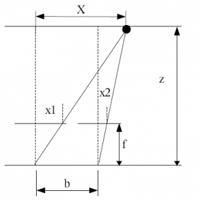
The principle behind stereometry is based on the human eye perception of depth. In humans, we perecieve depth by viewing the same object at two different angles (hence, two eyes). The lens in at position x=0 sees the object at X at different angle from x=b. Thus, by simple ratio and proportion, we can percieve depth z using the relation

where b is the separation distance of the lens, f is the focal length of the camera, and x2 and x1 are the location of the locations of the objects from the two different images.
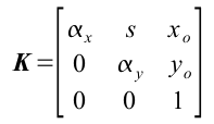
where  and
and  . However, if we are lucky enough, we may not need to compute for K if pertinent information such as f is given in the metadata of our camera. In our case, f=5.4mm. In any case, i still calculated K and found it to be
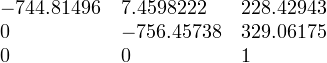
Note that xo=228 and y=329, which is near the center of a 480×640 image. Take note, however, that the image center may not be the 1/2 the image dimensions.
Reconstruction is done by getting as much (x,y) corresponding values in the two images. Take note that each point should have a correspondence in the other image. After which, bicubic spline splin2d and interpolation interp2d is done to create a smooth surface for our reconstruction.
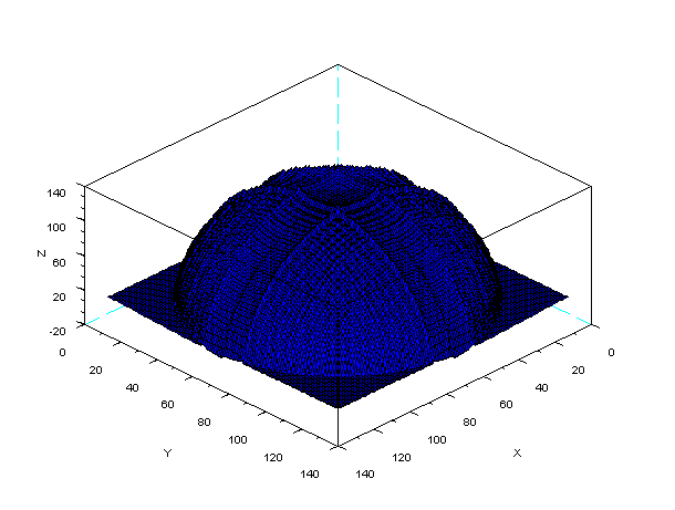
After reconstruction, we result in the following image. Although it may not actually be obvious at first glance, the resulting images do resemble the front and top facade of the rubix cube. Shown below are the reconstruction viewed from different angles (the thick black lines are aides in deciphering the shape of the object).
One of the obvious error in the reconstruction is the waviness of the surface. The reason for this is the finite number of points that we have chosen for reconstruction (in my case, 24) and the way splin2d and interp interpolates points in the mesh. Another possible error is the fact that our images are 2d and not 3d, and as such, any 2 points in the 3d object may have the same (x,y) coordinate in the image plane.
I want to give myself here a 9 because even though the reconstruction along the x seems flawed, i was able to extact depth (or z values) of the images.
Activity 13: Photometric Stereo
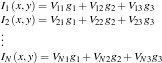
We consider a point light source from infinity located at  . The intensity
  as captured by the camera at image location (x,y) is proportional to the brightness
  . Thus we have

then
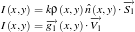
where
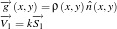
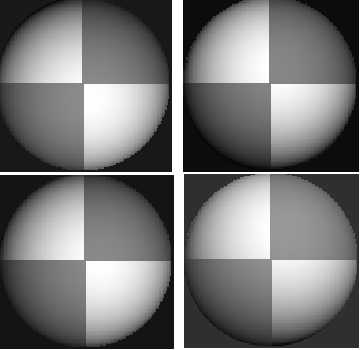
We can approximate the shape of an object by varying the light source and taking the picture of the image at various locations. The (x,y,z) of the light sources are stored in the matrix V.
Thus, we have
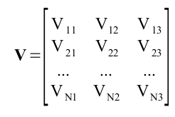
which are the the (x,y,z) locations of the N sources. The intensity for each point in the image is given by
or in matrix form

Since we know I and V, we can solve for g using

We get the normalize vectors using

After some manipulations we can compute the elevation z=f(x,y) using at any given (x,y) using
code:
loadmatfile(‘Photos.mat’);
V(1,: ) = [0.085832 0.17365 0.98106];
V(2,: ) = [0.085832 -0.17365 0.98106];
V(3,: ) = [0.17365 0 0.98481];
V(4,: ) = [0.16318 -0.34202 0.92542];
I(1, : ) = I1(: )’;
I(2, : ) = I2(: )’;
I(3, : ) = I3(: )’;
I(4, : ) = I4(: )’;
g = inv(V’*V)*V’*I;
g = g;
ag = sqrt((g(1,:).*g(1,: ))+(g(2,:).*g(2,: ))+(g(3,: ).*g(3,: )))+1e-6;
for i = 1:3
n(i,: ) = g(i,: )./(ag);
end
//get derivatives
dfx = -n(1,: )./(nz+1e-6);
dfy = -n(2,: )./(nz+1e-6);
//get estimate of line integrals
int1 = cumsum(matrix(dfx,128,128),2);
int2 = cumsum(matrix(dfy,128,128),1);
z = int1+int2;
plot3d(1:128, 1:128, z);
I give my self 10 points for this activity because there is high similarity in the shape of the actual object and photometric stereo.
Collaborators: Cole, Benj, Mark
