Activity 20: Neural Networks
A neural network is a mathematical model based on the workings of the human brains. It is composed of neurons arranged in layers that is fully connected with the preceding layer. The layers are called the input, hidden and output layers respectively. The input layer is where the input features are fed and forwarded to the hidden layer which is again forwarded to the output layer.

After the neurons are placed in the input, they are fed forward to the hidden neurons. The hidden neurons would have value  where
where  are the weights (strength of connection) association with the ith and hth neuron.
  is called the activation function because it mimics the the all-or-nothing firing of the neurons. Both hidden and output layers have activation functions given by


The tansig function is one of the most often used activation functions is pattern recognition problems. The output of the neural network is given by

where  is the weight associated with the hidden and output layers. The goal of NN is to minimize the error function E given by

where  is the actual output of the fed input pattern. This neural network is also called supervised neural network because you have an idea of what the output is. In a way, you can also look at it as forcing the NN to adjust weights such that a given input has the desired output.
The weights are updated as

where  is the weight at the qth iteration. A similar process is done for .
As a note, a neural network may have more than one output neuron. For a 3-class classification, we can have group A would output 0-0, group B would have 0-1 and group C would have 1-1. It is also important to normalize the inputs to between 0 and 1 because sigmoidal functions plateus at high values. That is, tansigmoidal of 100 is similar to tansigmoidal 200. Finally, the output of NN would not always be 1s or 0s. Thus, some sort of thresholding is done, like if the output is greater then 0.5 it is 1, otherwise 0.
For my classification my results are as follows.

This has accuracy of 93.3%. Also, the training set has 100% classification results. My code written in matlab is as follows:
net=newff(minmax(training),[25,2],{‘tansig’,’tansig’},’traingd’);
net.trainParam.show = 50;
net.trainParam.lr = 0.01;
%net.trainParam.lr_inc = 1.05;
net.trainParam.epochs = 1000;
net.trainParam.goal = 1e-2;
[net,tr]=train(net,training,training_out);
a = sim(net,training);
a = 1*(a>=0.5);
b = sim(net,test);
b = 1*(b>=0.5);
diff = abs(training_out – b);
diff = diff(1,:) + diff(2, :);
diff = 1*(diff>=1);
Activity 19: Linear Discriminant Analysis
Linear discriminant analysis is one of the simplest classification techniques to implement because it enables us to create a discriminant function from predictor variables. In this activity, i tried classifying between nova and piatos. The features i used where their RGB values and size.


The f values are given as follows
f1 f2
1 636.89 593.53
1 588.54 551.74
1 587.14 561.56
1 553.42 515.54
2 340.98 392.78
2 409.91 434.11
2 438.59 474.51
2 431.21 462.89
An object is assigned a class with the highest f value. As can be seen, most of group 1 have high f1 values while those in group 2 have higher f2 values.
As can be seen in our confusion matrix, we have 100% classification

Here is my code:
clear all;
chdir(‘/home/jeric/Documents/Acads/ap186/AC18’);
exec(‘/home/jeric/scilab-5.0.1/include/scilab/ANN_Toolbox_0.4.2.2/loader.sce’);
exec(‘/home/jeric/scilab-5.0.1/include/scilab/sip-0.4.0-bin/loader.sce’);
stacksize(4e7);
getf(‘imhist.sce’);
getf(‘segment.sce’);
training=[];
test=[];
prop=[];
loc=’im2/’;
f=listfiles(loc);
f=sort(f);
[x1, y1]=size(f);
for i=1:x1;
im=imread(strcat([loc, f(i)]));
im2=im2gray(im) ;
if max(im2)<=1
im2=round(im2*255);
end
[val, num]=imhist(im2);
im2=im2bw(im2, 210/255);
im2=1-im2;
ta=sum(im2); // theoretical area
[x,y]=find(im2==1);
temp=im(:,:,1);
red=mean(temp(x));
temp=im(:,:,2);
green=mean(temp(x));
temp=im(:,:,3);
blue=mean(temp(x));
prop(i,:)=[red, green, blue, ta];
end
max_a=max(prop(:,4));
max_r=max(prop(:,1));
max_g=max(prop(:,2));
max_b=max(prop(:,3));
prop(:,4) = prop(:,4)/max_a;
prop(:,1) = prop(:,1)/max_r;
prop(:,2) = prop(:,2)/max_g;
prop(:,3) = prop(:,3)/max_b;
training = prop(1:2:x1,:);
test = prop(2:2:x1, :);
m1 = mean(training(1:4,:),1);
m2 = mean(training(5:8,:),1);
training1 = training(1:4, :);
training2 = training(5:8,:);
training1 = training1 – mtlb_repmat(m1, 4,1);
training2 = training2 – mtlb_repmat(m2, 4,1);
//LDA
n1 = 4;
n2 = 4
c1 = (training1)’ * training1 / n1;
c2 = (training2)’ * training2 / n2;
c = 1./8*(4*c1+4*c2);
p = [1./2; 1./2];
for i = 1:8
f1(i) = m1*inv(c)*training(i,:)’ – 0.5*m1*inv(c)*m1’+log(p(1));
f2(i) = m2*inv(c)*training(i,:)’ – 0.5*m2*inv(c)*m2’+log(p(2));
if f1(i)>f2(i) then
class(i)=1;
else class(i)=2;
end
end
class
you may look take a look at http://people.revoledu.com/kardi/tutorial/LDA/LDA.html for a more thorough discussion of LDA.
Activity 18: Minimum Distance Classification
Pattern recognition techniques has long been studied by scientists for their potential applications. Human face recognition, coral reef analysis and gait analysis have been successful implentations of pattern recognition techniques.
One of the most basic forms of pattern recognition techniques is through attibutes of a given sample and compare it with the attributes of a training set. In this activity, we use different samples of chips, namely Chippy, Nova and Piatos and attempted to distinguish chips from each other through the attributes obtained form the training set.

Ten samples of each kind of chip was photographed with a camera. After which, cut each images to ascertain that a single image contains a single chip. Image processing techniques such segmentation was performed to remove the chip from the background. Afterwich the average value of the R, G and B of each chip was obtained as well as the area. The chip is then represented by the vector x containing the features of the chip. We do this for all chips in our training set. If we have W types of chips (chippy, nova, and piatos), we obtain the average feature vector of each class given by

for all j=1,2,..W.
The features of each test chip are obtained and the distance from each class is computed using

where

The test chip is classified based on the class with the minimum distance. Take note also that I normalized each vector to eliminate bias towards features whose values are extremely large (area for example) and eliminate bias against small numbers (R value for example).
Here is the confusion matrix of the test set of my 3-class classification. This is good enough with accuracy of 87%.

Activity 17: Basic Video Processing
Videos are becoming common with the advent of the digital era. Almost anyone can create their own videos. We can take advantage of this technology in exploring physics by performing experiments and monitor certain variables as a function of time.
A video is simply a string of still images flashed one after the other. The rate at which the video is captured is called the frame rate (measured in frames per second, fps). The higher the frame rate, the higher quality of the image in terms of smoothness of motion and time resolution. In our case, we used Cole’s web camera that can capture videos to see the dynamics of a physical pendulum (as opposed to a simple pendulem). His camera has frame rate of 15fps and, by Nyquist criterion, we can only resolve harmonic motion with frequency of less than 8Hz.
In this activity our group (me, cole and mark) decided that we want to invsitigate the period of a physical pendulum and compare it with theoretical predictions. For the first part, we captured video from the web cam and converted the frames to image files in *.jpg format (using avidemux) with the same fps but with reduced images size to 120 by 180 (from the original 480 by 720). The images were then subject to white balancing, chromaticity normalization, image segmentation (using color), binarization (using grayscale histogram), and opening and closing transformation. Basically we applied here everything we did for the entire sem. :). Assumptions regarding the ruler include homogeneity in the density of the ruler, the pivot is at excatly at the edge, and that the center of mass located exactly in the middle of the ruler.

Here is the gif animation i made (i converted the images to gif animation to avoid problems with the UP blocking access to video sharing sites such as youtube). The left is the orginal set of images, the middle are the normalized ones and the last are the binarized images. The gif is quite large (1.6mb) but once it gets loaded, it keeps on rolling. 🙂 I also ensured the the speed of the gif is similar to the fps of the camera used.
A physical pendulum is a more generalized pendulum with no ideal strings. The period of oscillation of this pendulum is given by

where I is the moment of inertia about the pivot and L is the distance of the center of mass from the pivot. 
For our ruler with length h and width w with pivot around the end the moment of inertia is given by

The period of oscillation can be obtained from the graph by plotting the location of the center of mass as a function of time and getting the distance between two peaks.If this is what we use, we get a period of 1.2 sec

I also used fft to get the dominating frequency of our signal above, and found it to 0.769 Hz or a period of around 1.3 sec which is not far from the above. I also believe that the frequency obtained by fft is more accurate than just picking peaks. 🙂

Theoretically, this ruler with mass 174.8g, length of 63.5cm and width of 3cm would have a period of oscillation of 1.31s (the moment of inertia being 0.0235). This means we have error of only 0.76%. This is very near the expected value , considering that the we had a few assumptions regarding this ruler.
-oOo-


-oOo-
Here are the functions i made that were invoked above.
closing.sce

open.sce

imhist.sce

segment.sce

white_balance.sce

-oOo-
Collaborators: Mark, Cole
I want to give myself a 10 here because i believe I was able to complete what has to be done by applying almost everything we had learned.:)
Activity 16: Image Segmentation
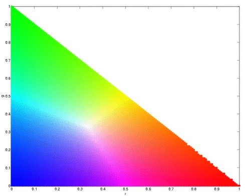
Segmentation (choosing of objects in colored images) is useful in many aspects of digital image processing like face detection. More often than not, an object would have one color, for example, a mug or a ball, or hand. However, lighting variations may affect the luminosity of our images and as such, we must remove these luminosity attributes in processing our images. To remove luminosity effects we normalized each channel to
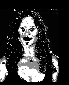
where  . We then crop a portion of the object (regions of interest, ROI) that we will segment and use this as a “model” from which certain parameters will be obtained. If our object is more or less monochromatic, it will more or less cover a small blob in our chromaticity diagram (figure above). We then. Here, we have a picture of Catherin Zeta-Jones taken from: http://www.latest-hairstyles.com/

Our “model” is a patch form here neck down to her bust to gather as much colors as possible.
Parametric Probability Distribution
We assume that the distribution of colors in our ROI are normally distributed where the mean and the variance we obtain from our “model” cropped images. The probability that the red channel of a pixel is belonging to the red component of the “model” is given by
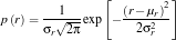
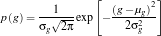
where  and
and  are the mean and standard deviation respectively. The probability that a pixel belongs to the “model” is a joint probability given by

We perform this over all pixels and plot the probability that a pixel belongs to our ROI.
Here is our distrution but is not yet normalized.
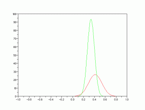
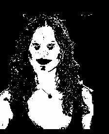
We obtained the joint probability distribution and used “imshow” to plot the probability that a pixel belongs to our ROI. As we can see, most of her torso, face and neck is colored almost white, which means there is high probability that hey belong to our ROI. And advantage of this method is it is more robust when it comes to color of the ROI not belonging to the “model”.
Non-parametric Probability Distribution (Histogram Backprojection)
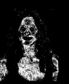
The next method is through histogram backprojection. In this method, we used a normalized chromaticity distribution histogram (obtained from the “model”) with 32 bins along the red and green. The histogram of the model is shown below.
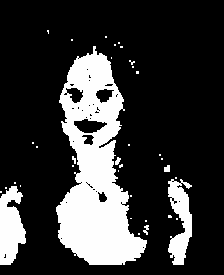
This method works by getting the r and g values of a pixel and locates the probabilty that it belongs to the “model”. It replaces the pixel value with the probility of the pixel r-g values. The reconstruction is shown below.
As can be seen, this has better segmentation of the face, torso and arms. Another advantage of this method is it doesn’t assume normality of distribution unlike parametric one.
<!–
Extra Extra!
Furthermore, I applied what we have learned in Activity 3 and Activity 9 in this activity. I threshold the image to get a black and white image, resulting to this:
Looking closely, there are speckles in the hair, so i improved it by opening transformation and obtained this image
–>
-oOo-
clear all;
stclear all;
stacksize(4e7);
chdir(‘/home/jeric/Documents/Acads/ap186/a16’);
ROI=imread(‘face.jpg’);
I=ROI(:,:,1)+ROI(:,:,2)+ROI(:,:,3);
I(find(I==0))=100;
ROI(:,:,1)=ROI(:,:,1)./I;
ROI(:,:,2)=ROI(:,:,2)./I;
ROI(:,:,3)=ROI(:,:,3)./I;
ROI_sub=imread(‘face_cropped.jpg’);
I=ROI_sub(:,:,1)+ROI_sub(:,:,2)+ROI_sub(:,:,3);
ROI_sub(:,:,1)=ROI_sub(:,:,1)./I;
ROI_sub(:,:,2)=ROI_sub(:,:,2)./I;
ROI_sub(:,:,3)=ROI_sub(:,:,3)./I;
//probability estimatation
mu_r=mean(ROI_sub(:,:,1)); st_r=stdev(ROI_sub(:,:,1));
mu_g=mean(ROI_sub(:,:,2)); st_g=stdev(ROI_sub(:,:,2));
Pr=1.0*exp(-((ROI(:,:,1)-mu_r).^2)/(2*st_r^2))/(st_r*sqrt(2*%pi));
Pg=1.0*exp(-((ROI(:,:,2)-mu_g).^2)/(2*st_g^2))/(st_r*sqrt(2*%pi));
P=Pr.*Pg;
P=P/max(P);
scf(1);
x=[-1:0.01:1];
Pr=1.0*exp(-((x-mu_r).^2)/(2*st_r))/(st_r*sqrt(2*%pi));
Pg=1.0*exp(-((x-mu_g).^2)/(2*st_g))/(st_g*sqrt(2*%pi));
plot(x,Pr, ‘r-‘, x, Pg, ‘g-‘);
scf(2);
imshow(P,[]);
//roi=im2gray(ROI);
//subplot(211);
//imshow(roi, []);
//subplot(212);
//<————-histogram backprohection————————————>
//histogram
r=linspace(0,1, 32);
g=linspace(0,1, 32);
prob=zeros(32, 32);
[x,y]=size(ROI_sub);
for i=1: x
for j=1:y
xr=find(r<=ROI_sub(i,j,1));
xg=find(g<=ROI_sub(i,j,2));
prob(xr(length(xr)), xg(length(xg)))=prob(xr(length(xr)), xg(length(xg)))+1;
end
end
prob=prob/sum(prob);
//show(prob,[]); xset(“colormap”, hotcolormap(256));
scf(3)
surf(prob);
//backprojection
[x,y]=size(ROI);
rec=zeros(x,y);
for i=1: x
for j=1:y
xr=find(r<=ROI(i,j,1));
xg=find(g<=ROI(i,j,2));
rec(i,j)=prob(xr(length(xr)), xg(length(xg)));
end
end
scf(4);
imshow(rec, []);
rec=round(rec*255.0);
getf(‘imhist.sce’);
[val, num]=imhist(rec);
scf(5);
plot(val, num);
scf(6);
rec=im2bw(rec, 70/255);
imshow(rec, []);
//opening
se=ones(3,3);
im=rec;
im=erode(im, se);
im=dilate(im, se);
scf(7);
imshow(im, []);
-oOo-
I give myself a 10 here because I did well in segmenting the images. 🙂
Activity 15: White Balancing
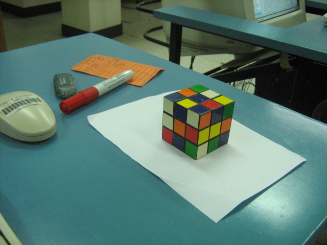
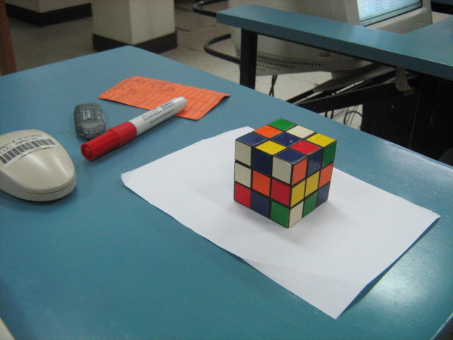
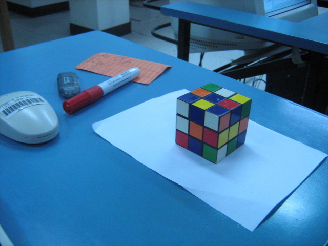
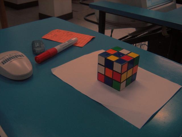
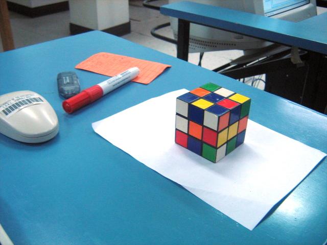
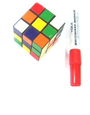
White balancing is a technique wherein in images captured under lighting conditions are corrected such that white appears white. It may not really be obvious (since the eyes have white balancing capabilities) unless we compare the object with the image itself. Here is an image of a rubix cube take under different white-balancing conditions in a room with fluorescent light.
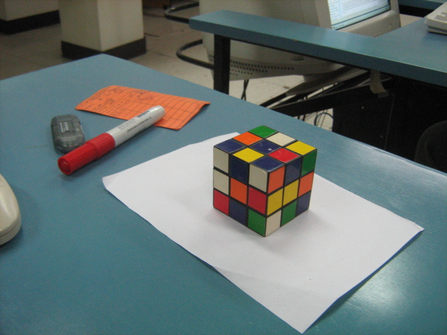
Automatic white balancing.
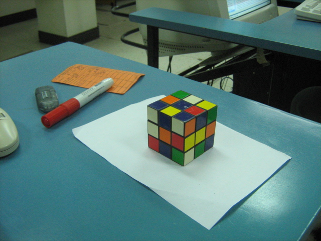
cloudy, daylight and fluorescent white balancing
tungsten white balancing
From the images above, we can see that if you just used any white balance, we may not get the desired image. And can be seen in the case of tungsten, white doesn’t appear white.This can be corrected via white balancing methods. There are two methods that can be used in performing white balancing, namely, the Reference White and the Gray World algorithm.
Let’s start with the basic. A digital image is composed of an MxNx3 matrix where MxN is the dimension of the image and there are 3 channels for that image. Each channel corresponds to one of the three primary colors namely red, green and blue. A pixel then is contains the information about the amount of red, green and blue in that channel. The reference white algorithm works by choosing a white object in the image and getting it’s RGB values. This is used as reference for determining which is “white” in the image. The red channels of each pixel is divided by the red value of the reference white object. The same is done for all other channels. The gray world algorithm on the other hand works by assuming the image is gray (ie, each pixel has equal R-G-B values).The gray world algorithim is implemented by averaging the R-G-B of each channel in the unbalanced image. The red channel of the unbalanced image is then divided by the R above. The same is done for the blue and green channels. If a channel exceeds 1.0 on any pixel, it is cut-off to 1.0 to avoid saturation.
Here is the result of white balancing using the gray world algo (left) and the reference white (right). As can be seen here, can see that reference white is superior in terms of image quality. The problem with GWA is that averaging channels puts bias to colors that are not abundant. In our case, there is bias against the green.
Here we tried to implement GWA and RW by making the background white to ensure more or less the same amount of colors present.
Here is the results for GWA (left) and RF (right). The rendering of white of GWA is OK, and is close to the actual image. On the other hand, the RF method produced a very brightly colored image. Now, we can see that a disadvantage of RF is that it relies on what should be white and is highly subjective then. A problem would exist in RF if there are no white objects in the image (or if a reference white is not exactly white).
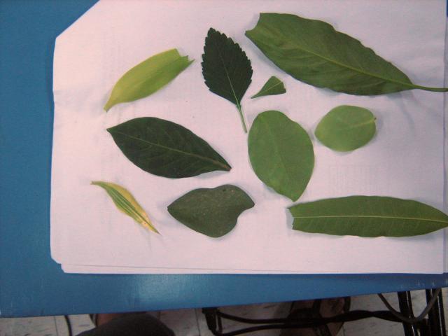
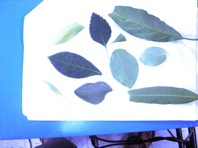
Here we used many shades of green in performing white balancing.
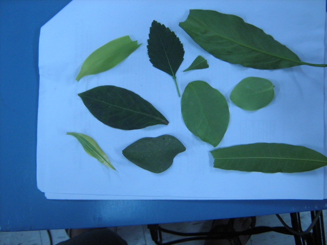
We can see that the GWA produced better results than RF. Again, RF saturated with the white.
I give myself a 10 for this activity.
-oOo-
clear all;
stacksize(4e7);
name=’leaf_and_all 001‘
im=imread(strcat(name + ‘.jpg’));
//imshow(im);
//[b,xc,yc]=xclick()
//reference white
x=124;
y=184;
r=im(x,y,1);
g=im(x,y,2);
b=im(x,y,3);
im1=[];
im1(:,:,1)=im(:,:,1)/r;
im1(:,:,2)=im(:,:,2)/g;
im1(:,:,3)=im(:,:,3)/b;
g=find(im1>1.0);
im1(g)=1.0;
imwrite(im1, strcat(name + ‘rw.jpg’));
//imshow(im,[]);
//grayworld
r=mean(im(:,:,1));
g=mean(im(:,:,2));
b=mean(im(:,:,3));
im2=[]
im2(:,:,1)=im(:,:,1)/r;
im2(:,:,2)=im(:,:,2)/g;
im2(:,:,3)=im(:,:,3)/b;
im2=im2/max(im2);
g=find(im2>1.0);
im2(g)=1.0;
imwrite(im2, strcat(name + ‘gw.jpg’));
//imshow(im,[]);
Activity 14: Stereometry
here is the RQ factorization code from: http://www.cs.nyu.edu/faculty/overton/software/uncontrol/rq.m written by Michael Overton and modified by yours truly for scilab.
-oOo-
function [R,Q]= rq(A)
//% full RQ factorization
//% returns [R 0] and Q such that [R 0] Q = A
//% where R is upper triangular and Q is unitary (square)
//% and A is m by n, n >= m (A is short and fat)
//% Equivalent to A’ = Q’ [R’] (A’ is tall and skinny)
//% [0 ]
//% or
//% A’P = Q'[P 0] [P R’ P]
//% [0 I] [ 0 ]
//% where P is the reverse identity matrix of order m (small dim)
//% This is an ordinary QR factorization, say Q2 R2.
//% Written by Michael Overton, overton@cs.nyu.edu (last updated Nov 2003)
m = size(A,1);
n = size(A,2);
if n < m
error(‘RQ requires m <= n’)
end
P = mtlb_fliplr(mtlb_eye(m));
AtP = A’*P;
[Q2,R2] = qr(AtP);
bigperm = [P zeros(m,n-m); zeros(n-m,m) mtlb_eye(n-m)];
Q = (Q2*bigperm)’;
R = (bigperm*R2*P)’;
-oOo-
you can invoke the function by saving the file as ‘rq.sce’ and invoking at using getf(‘rq.sce’);
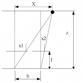
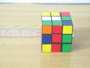
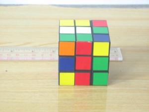
The principle behind stereometry is based on the human eye perception of depth. In humans, we perecieve depth by viewing the same object at two different angles (hence, two eyes). The lens in at position x=0 sees the object at X at different angle from x=b. Thus, by simple ratio and proportion, we can percieve depth z using the relation

where b is the separation distance of the lens, f is the focal length of the camera, and x2 and x1 are the location of the locations of the objects from the two different images.
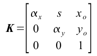
where  and
and  . However, if we are lucky enough, we may not need to compute for K if pertinent information such as f is given in the metadata of our camera. In our case, f=5.4mm. In any case, i still calculated K and found it to be

Note that xo=228 and y=329, which is near the center of a 480×640 image. Take note, however, that the image center may not be the 1/2 the image dimensions.
Reconstruction is done by getting as much (x,y) corresponding values in the two images. Take note that each point should have a correspondence in the other image. After which, bicubic spline splin2d and interpolation interp2d is done to create a smooth surface for our reconstruction.
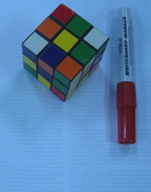
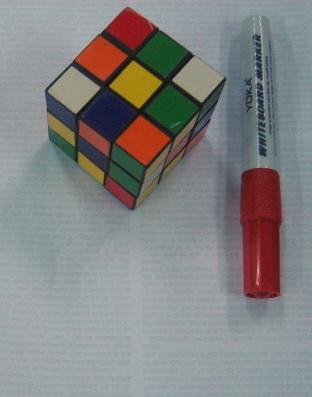
After reconstruction, we result in the following image. Although it may not actually be obvious at first glance, the resulting images do resemble the front and top facade of the rubix cube. Shown below are the reconstruction viewed from different angles (the thick black lines are aides in deciphering the shape of the object).
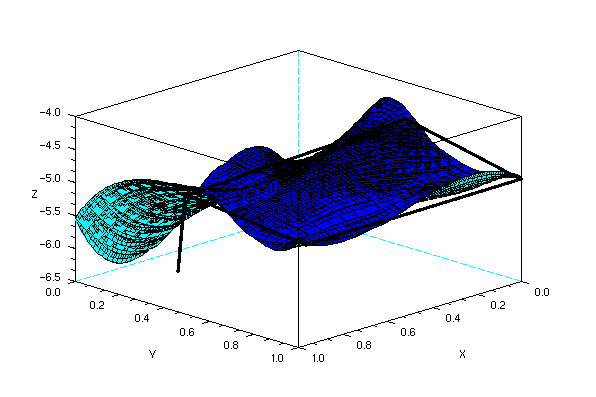
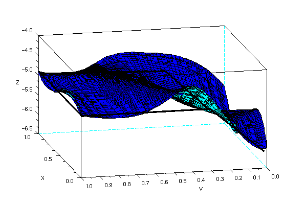
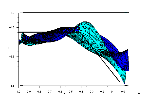
One of the obvious error in the reconstruction is the waviness of the surface. The reason for this is the finite number of points that we have chosen for reconstruction (in my case, 24) and the way splin2d and interp interpolates points in the mesh. Another possible error is the fact that our images are 2d and not 3d, and as such, any 2 points in the 3d object may have the same (x,y) coordinate in the image plane.
I want to give myself here a 9 because even though the reconstruction along the x seems flawed, i was able to extact depth (or z values) of the images.
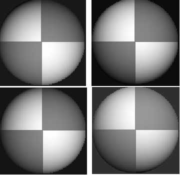
Activity 13: Photometric Stereo
We consider a point light source from infinity located at  . The intensity
  as captured by the camera at image location (x,y) is proportional to the brightness
  . Thus we have

then
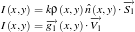
where
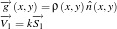
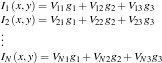
We can approximate the shape of an object by varying the light source and taking the picture of the image at various locations. The (x,y,z) of the light sources are stored in the matrix V.
Thus, we have
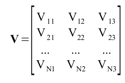
which are the the (x,y,z) locations of the N sources. The intensity for each point in the image is given by
or in matrix form

Since we know I and V, we can solve for g using

We get the normalize vectors using

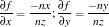
After some manipulations we can compute the elevation z=f(x,y) using at any given (x,y) using
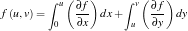
code:
loadmatfile(‘Photos.mat’);
V(1,: ) = [0.085832 0.17365 0.98106];
V(2,: ) = [0.085832 -0.17365 0.98106];
V(3,: ) = [0.17365 0 0.98481];
V(4,: ) = [0.16318 -0.34202 0.92542];
I(1, : ) = I1(: )’;
I(2, : ) = I2(: )’;
I(3, : ) = I3(: )’;
I(4, : ) = I4(: )’;
g = inv(V’*V)*V’*I;
g = g;
ag = sqrt((g(1,:).*g(1,: ))+(g(2,:).*g(2,: ))+(g(3,: ).*g(3,: )))+1e-6;
for i = 1:3
n(i,: ) = g(i,: )./(ag);
end
//get derivatives
dfx = -n(1,: )./(nz+1e-6);
dfy = -n(2,: )./(nz+1e-6);
//get estimate of line integrals
int1 = cumsum(matrix(dfx,128,128),2);
int2 = cumsum(matrix(dfy,128,128),1);
z = int1+int2;
plot3d(1:128, 1:128, z);
I give my self 10 points for this activity because there is high similarity in the shape of the actual object and photometric stereo.
Collaborators: Cole, Benj, Mark
Activity 12: Correcting Geometric Distortions (partial)
*note. i still have to implement grayscale interpolation. as of the moment, i only did the pixel coordinate correction.
We can imagine our image as if it was warped through some linear transformation.
![]()
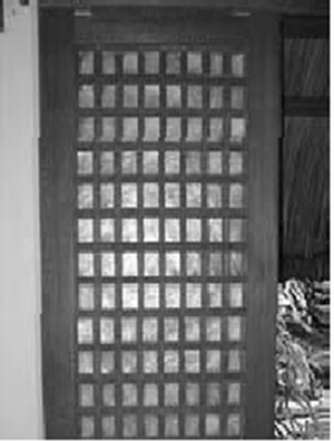
To better visualize the problem, we assume that we have a straight grid as pictured in the right side of the above image. However, since the camera has inherent geometrical aberrations, the picture we image would be warped and transformation is given as


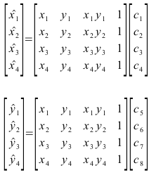
where x’ and y’ are the coordinates of the pixels x,y (orig image) in the distorted image. Further, we assume that the transformation is is that of a bilinear function as shown below.


Thus, we have the transformation function as
![]()
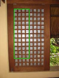
The values of c are determined from the four vertices of corresponding polygon in the distorted image and ideal image. In this activity, I highlighted my region of interest and measured the actual and ideal pixel location of the region of interest. The green-highlighted section is the ideal locations of the grids.
However, the values of  and
and  are valid in the included polygon.
My code below was executed from this set of instructions (from Dr Soriano’s lecture).
1. Obtain image.
2. From the most undistorted portion of the image, e.g. at the optical axis of the camera, count the number of pixels down and across one box.
3. Generate the ideal grid vertex points (just the coordinates).
4. For each rectangle compute c1 to c8 using pairs of equations (x’s,y’s) from the four corner points.
In compact matrix form, we have  and
and  . We can solve for the c’s using
 and
and  .
.
5. Per pixel in the ideal rectangle, determine the location of that point in the distorted image using
![]()
6. If the computed distorted location is integer-valued, copy the grayscale value from the distorted image onto the blank pixel. If the location is not integer-valued, compute the interpolated grayscale value using:

im=imread(‘image.jpg’);
im=im2gray(im);
[x,y]=size(im);
ideal=zeros(x,y);
for i=1 : 10 : x
ideal(i, :)=ones(y);
end
for j=1:8:y
ideal(:, j)=ones(x);
end
scf(1);
imshow(ideal, []);
blank=[];
xi=[31; 183; 183; 31];
yi=[48; 50; 97; 95];
T=[31 48 31*48 1; 245 48 245*48 1; 245 95 145*95 1; 31 95 31*95 1];
c14=inv(T)*xi;
c56=inv(T)*yi;
for i=1 : x
for j=1:y
x_im=c14(1)*i+c14(2)*j+c14(3)*i*j+c14(4);
y_im=c56(1)*i+c56(2)*j+c56(3)*i*j+c56(4);
if x_im>=x
x_im=x;
end
if y_im>=y
y_im=y;
end
blank(i, j)=im(round(x_im), round(y_im));
end
end
scf(2);
imshow(blank, []);
//for j=1:10:y
// ideal(:, y)=ones(x);
//end
Activity 11: Camera Calibration
In this activity, we calibrate a camera to determine the mapping of each location (3D) on an object to its camera image (2D). This is shown in the figure below from Dr Soriano’s lecture.
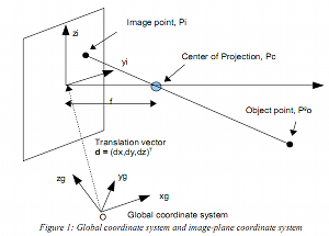
After some algebra, we are lead to this equation where the “o” subscript refer to the object and the “i” subscript refer to the image. As can be seen, the there are only two equation for the mapping since the image is flat.
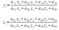
In matrix form, the above equation is written as
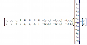
However, this is for a single image, and we have to append the Q and d matrix as we increase the number of points that will be used to determine the mapping. In compact matrix form, we have
We can solve for the transformation matrix a using some matrix algebra which results to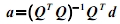
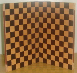
The image that we have obtained by taking a picture of the checker board is shown below. The location of the points used in determining the mapping is shown in my program.
x=[0 0 0 0 1 1 2 0 1 0 3 1 0 3 0 2 0 0 0 1 ];
y=[0 1 0 3 0 0 0 1 0 5 0 0 2 0 2 0 5 3 0 0 ];
z=[0 12 3 2 1 2 5 8 1 3 8 9 6 10 7 7 9 10 9];
yi=[127 139 126 164 115 115 102 139 113 191 90 114 152 88 152 101 193 166 125 112];
zi=[200 187 169 161 172 189 175 123 73 200 161 73 57 112 40 91 97 58 138 56];
obj=[];
im=[];
for i=0:length(x)-1
obj(2*i+1, :)=[x(i+1) y(i+1) z(i+1) 1 0 0 0 0 -yi(i+1).*x(i+1) -yi(i+1).*y(i+1) -yi(i+1).*z(i+1)];
obj(2*i+2, :)=[0 0 0 0 x(i+1) y(i+1) z(i+1) 1 -zi(i+1).*x(i+1) -zi(i+1).*y(i+1) -zi(i+1).*z(i+1)];
im(2*i+1)=yi(i+1);
im(2*i+2)=zi(i+1);
end
a=inv(obj’*obj)*obj’*im;
a(12)=1.0;
a=matrix(a, 4, 3)’;
testx=1;
testy=0;
testz=2;
ty=(a(1,1)*testx+a(1,2)*testy+a(1,3)*testz+a(1,4))/(a(3,1)*testx+a(3,2)*testy+a(3,3)*testz+a(3,4));
tz=(a(2,1)*testx+a(2,2)*testy+a(2,3)*testz+a(2,4))/(a(3,1)*testx+a(3,2)*testy+a(3,3)*testz+a(3,4));
ty
tz
We’ve verified that this works with error of a few pixels. As of the moment, more accurate methods of getting the points is needed for a more accurate calibration. In our data, the actual pixel values of (1,0,2) are (114, 172) while the value from the calibration is (122, 177). A possible source of error, other than inaccuracy in getting the pixel values is radial distortion (as was mentioned by Dr Soriano). Another source of error is the high resolution of the image which causes error in choosing which pixel is the corner of the board.
I give my self 9.5/10 because of some inaccuracies encountered. Although i am satisfied enough with the result.
Tnx to Julie for the help with the image. 🙂
